embedding_2d_plot

Plot a 2D embedding (e.g., t-SNE, PCA, UMAP) colored by categorical groups or continuous values, with optional density contours, legends, and colorbars.

---

📥 Arguments

Name	Type	Required	Description
df	pd.DataFrame	✅	DataFrame containing at least ‘x’, ‘y’, and the hue column.
font_family	str	❌	Font family for title, legend, and colorbar. Default: ‘Times New Roman’.
title	str	❌	Title for the plot. Default: None.
mode	str	❌	Plotting mode: ‘categorical’ or ‘continuous’. Default: ‘categorical’.
hue_column	str	❌	Column name for coloring points. Must be provided.
palette	List[str]	❌	List of colors for categorical groups. If None, uses seaborn ‘tab20’ palette.
cmap_continuous	str	❌	Matplotlib colormap name for continuous values. Default: ‘viridis’.
display_legend	bool	❌	Whether to display the legend (categorical mode only). Default: False.
legend_loc	str	❌	Legend location if displayed. Default: ‘lower right’.
display_cbar	bool	❌	Whether to display the colorbar (continuous mode only). Default: False.
cbar_loc	str	❌	Colorbar inset location if displayed. Default: ‘lower right’.
show_density	bool	❌	Whether to overlay density contours (continuous mode only). Default: False.
density_column	str	❌	Column to use for density grouping. Default: ‘island’ if exists.
density_alpha	float	❌	Transparency for density contours. Default: 0.5.
figsize	tuple	❌	Figure size in inches. Default: (8, 8).
s	int	❌	Marker size for scatter points. Default: 40.
alpha	float	❌	Transparency for scatter points. Default: 0.9.
edgecolor	str	❌	Edge color for scatter points. Default: ‘white’.
linewidth	float	❌	Edge line width for scatter points. Default: 0.3.
save	str	❌	Base filename to save PNG and PDF versions if provided.

---

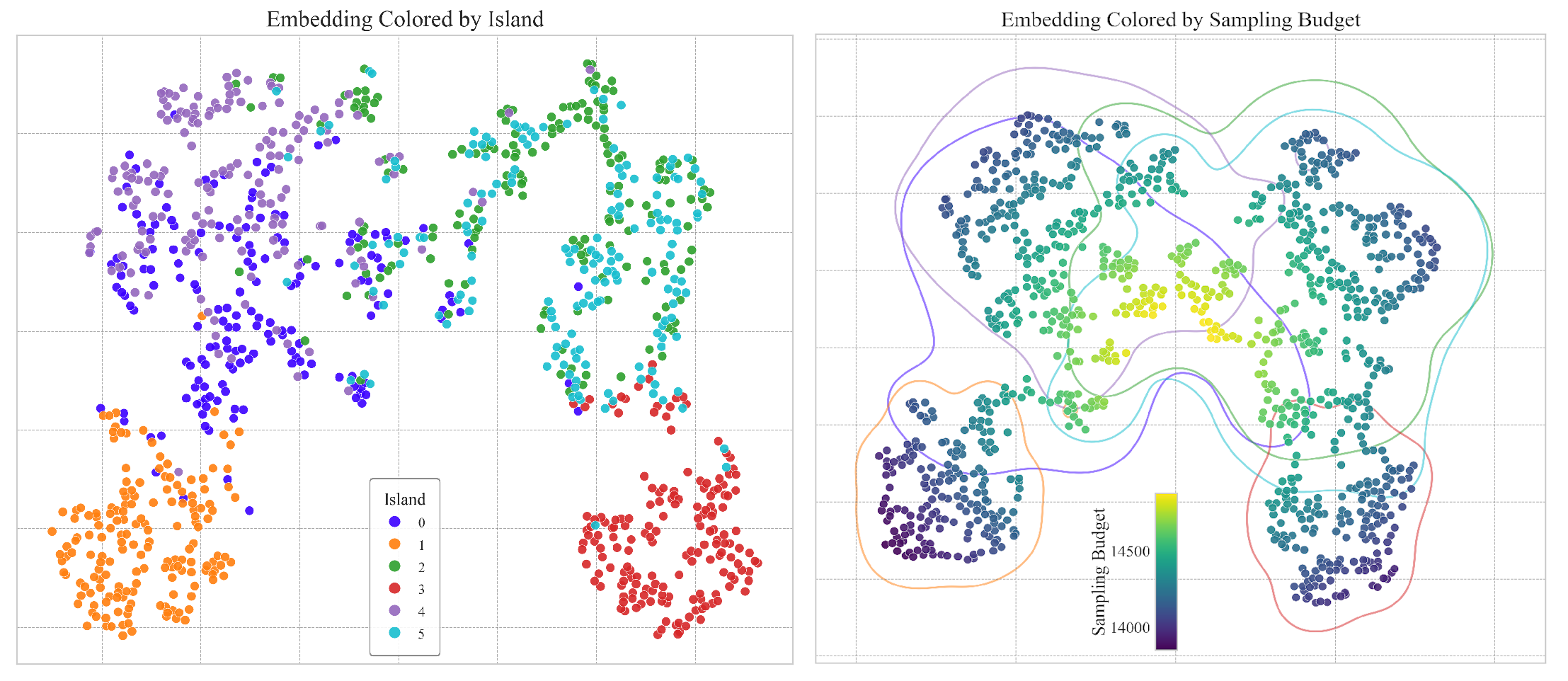
📦 Example Output

Click to show example code

import numpy as np
from matplotlib import pyplot as plt
import pandas as pd
from sklearn.datasets import make_blobs
from sklearn.manifold import TSNE
from swizz import plot

# 1. Create clustered data
X, y = make_blobs(
    n_samples=1000,
    centers=6,
    cluster_std=2.2,  # Small but not tiny std: they overlap a little
    random_state=43
)

# Add tiny noise
X += np.random.normal(0, 0.5, X.shape)

# 1.2. Apply t-SNE
X_embedded = TSNE(n_components=2, random_state=42, perplexity=30).fit_transform(X)

# 1.3. Build structured sampling budget (just for example to make a case for the continuous example)
sampling_budget = 15000 - 4000 * np.tanh(np.linalg.norm(X_embedded, axis=1) / 150)

df = pd.DataFrame({
    "x": X_embedded[:, 0],
    "y": X_embedded[:, 1],
    "Island": y,
    "Sampling Budget": sampling_budget
})

# ---- 2. Plot: Categorical Mode (Island Coloring) ----

plot("embedding_2d_plot",
     df=df,
     mode="categorical",
     hue_column="Island",
     title="Embedding Colored by Island",
     display_legend=True,
     palette=[
         "#3b00ff", "#ff7f0e", "#2ca02c",
         "#d62728", "#9467bd", "#17becf"
     ],
     legend_loc="lower center",
     )
plt.show()

# ---- 3. Plot: Continuous Mode (Sampling Budget Coloring) ----

plot("embedding_2d_plot",
     df=df,
     mode="continuous",
     hue_column="Sampling Budget",
     density_column="Island",
     title="Embedding Colored by Sampling Budget",
     show_density=True,
     display_cbar=True,
     palette=[
         "#3b00ff", "#ff7f0e", "#2ca02c",
         "#d62728", "#9467bd", "#17becf"
     ],
     cbar_loc="lower center",
     )
plt.show()